A Pattern for Scaling the Value Proposition of LLMs: Ensemble and Distil 🚀

In our previous post we showed that Large Language Models (LLM) including PaLM-2, Gemini, and GPT-4 are able to assign sentiment labels with exceptional accuracy. We also showed that they massively outperform previous state of the art models like FinBERT. But it wasn't all good news. Using LLMs to label a corpus of 10 million news stories would cost thousands of dollars, take weeks to finish, and would be nearly impossible to scale to near-real-time use cases.

Which brings us to the inevitable question that goes through every person's mind when they attempt to scale the capabilities of Large Language Models ...

Well, sh*t! Now what?

Fortunately, there is a widely used pattern in data science that can help. I like to call it "ensemble and distil". Here's how it works in simple terms:

1. Curate a dataset representative of your whole corpus.
2. Label that dataset using a mix of large language models.
3. Ensemble the models to create a teacher model.
4. Distil the capability of the teacher into a student model.
5. Scale the student model to the rest of your corpus.

In this post we will show you how this is done. But, more importantly, we will explain why this ought to be done. At the risk of spoiling the surprise, we will also show that a simple linear regression trained to emulate the outputs of an LLM-ensemble from off-the-shelf sentence transformer embeddings can outperform GPT-4 at sentiment classification! Yeah, you read that right.

Before we get into the details, I want to use this opportunity to say a public thank you to Moabi Mokhoro and Deon van Heerden. During their machine learning internship at Nosible they worked on this project and taught us a lot.

Background

In the previous post we discussed the first and second step. If you have the time, I recommend reading it for added context. But here's a quick recap.

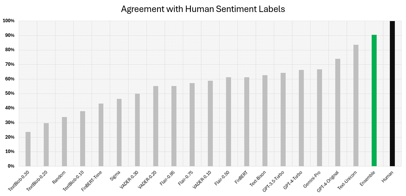
We curated a dataset of 10,378 news stories from our corpus. This dataset has news stories from all years, all industries, and all news categories. Next, we evaluated a variety of sentiment classification models on this dataset. These included: TextBlob, VADER, Flair, SigmaFSA, FinBERT, FinBERT-Tone, Bison, Unicorn, Gemini-Pro, GPT-3.5-Turbo, GPT-4, and GPT-4-Turbo.

Using human agreement as our measure of success we observed that the top three models were: Unicorn (84%), GPT-4 (74%), and Gemini-Pro (67%).

The Teacher

The goal of ensembling is to combine multiple models to create a new model that is more capable than any model individually. This does not always happen. More often than not, an ensemble of models is likely to produce a mediocre result. For the ensemble to be better than the best model, the stars need to align.

First, the individual models must be better than random. Second, the models must be correlated when they are right. And third, the models must be uncorrelated when they are wrong. If, and only if, these stars align is there a chance that an ensemble will be better than the best. Techniques like boosting, which train models on the errors of other models, do this explicitly.

One trick I like to use when building ensembles is iterative addition. This is a greedy procedure that starts off with the best model and then iteratively includes the most "additive" model until no more models are additive. Additive models are ones that improve the accuracy of the ensemble at each point.

When applied to the sentiment models this is what we got:

• Start with Unicorn (83.6%)
  • Then add GPT-3.5 (+2.80% boost)
    • Then add GPT-4 (+2.00% boost)
      • Then add SigmaFSA (+1.60% boost)
        • Then add Bison (+0.40% boost)

The resulting ensemble ends up with an agreement ratio of 90.4% with human labels. That is 6% better than the best model (Unicorn) in absolute terms. Because iterative addition is extremely quick, you can repeat this multiple times over a sample of your data to arrive at a probability distribution over the possible ensembles. Doing this is a useful test for overfitting risk.

Across 1,000 simulations this ensemble was the best 51% of the time. The next best ensemble was the same except that it excluded Bison. That was the best 13.8% of the time. And, finally, the third best ensemble was the same except that it included TextBlob-0.30. That was the best 11% of the time. Which is all just to say, we're confident that this is, in fact, the best ensemble.

There you have it, our teacher will be an ensemble that aggregates the outputs of Unicorn, GPT-3.5, GPT-4, SigmaFSA, and Bison. In order to get discrete labels from this ensemble we threshold it such that any aggregates greater than 1 are "Positive". Any aggregates less than -1 are "Negative". And anything in between is "Neutral". The goal is now to get our students to emulate the teacher.

The Students

To keep things nice and simple, all of the students in our experiment are simple ordinary least squares regression models. Over the years I've found that a linear regression fitted on good features is always hard to beat. Linear regression just works. It's also efficient, portable, and generalizes well. The only difference between each student was the input data they were fitted on.

For our students to learn from the teacher, we need to give them something to learn from. In the spirit of keeping with the student-teacher analogy, let's call that the "textbook". In 2024 the best textbook for our students to learn from are sentence embeddings from pretrained transformer models.

In the process of learning how to solve a natural language problem, neural networks transform the sentences they are given into sets of numbers. These sets of numbers are called embeddings or vectors, and they are the network's internal representation of the sentences. Embedding is a superpower of neural networks because it allows us to turn variable length sentences into fixed length vectors that capture a great deal of the information contained in the sentence.

The biggest challenge now is finding the right embedding model. Every week more models appear on the Massive Text Embedding Benchmark Leaderboard making it harder to navigate. Luckily for you, we look at it often and had a good idea which sentence transformers we wanted to evaluate for this blog post.

The Results

We ended up with 38 models in this survey. These included the teacher, the 7 LLMs we evaluated last week, and 30 ordinary least squares regression students that were trained to emulate the outputs of the teacher using various sentence transformer embeddings. The student models are denoted by OLS(name-of-sentence-transformer) to make it obvious what's what.

One unsurprising result was that the students fitted on embeddings from larger sentence transformer models did better than the students fitted on embeddings from smaller sentence transformer models. More surprisingly, when we looked at the data, we noticed that the E5 models from Microsoft were consistently "punching about their weight" in every class. Here's what I mean:

• Best with <100Mn parameters? e5-small-v2
• Best with 100Mn to 200Mn parameters? e5-base-v2
• Best with 300Mn to 400Mn parameters? e5-large-v2

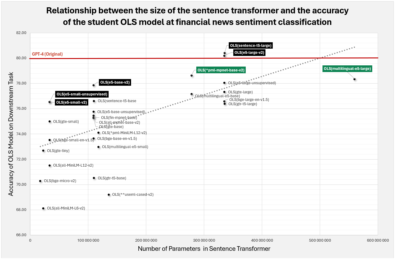
Even more surprisingly were how well the unsupervised versions of the E5 sentence transformers performed. We thought there would be a big difference between the two versions, but the differences were almost insignificant. Going forward we will be using the multilingual-e5-large embeddings. For more information on these models, please see this paper from Microsoft:

"Text Embeddings by Weakly-Supervised Contrastive Pre-training" by Liang Wang, Nan Yang, Xiaolong Huang, Binxing Jiao, Linjun Yang, Daxin Jiang, Rangan Majumder, and Furu Wei.

Because that's quite a lot of models we've broken up the results into the following categories - models with 384-dimensional vectors, models with 768-dimensional vectors, models with 1024-dimensional vectors, and multilingual models with either 384, 768, or 1024-dimensional vectors. Each result table shows the type of model, the number of likes on Hugging Face, the number of downloads on Hugging Face, and the out-of-sample accuracy versus the Teacher model.

384-Dimensional Vectors

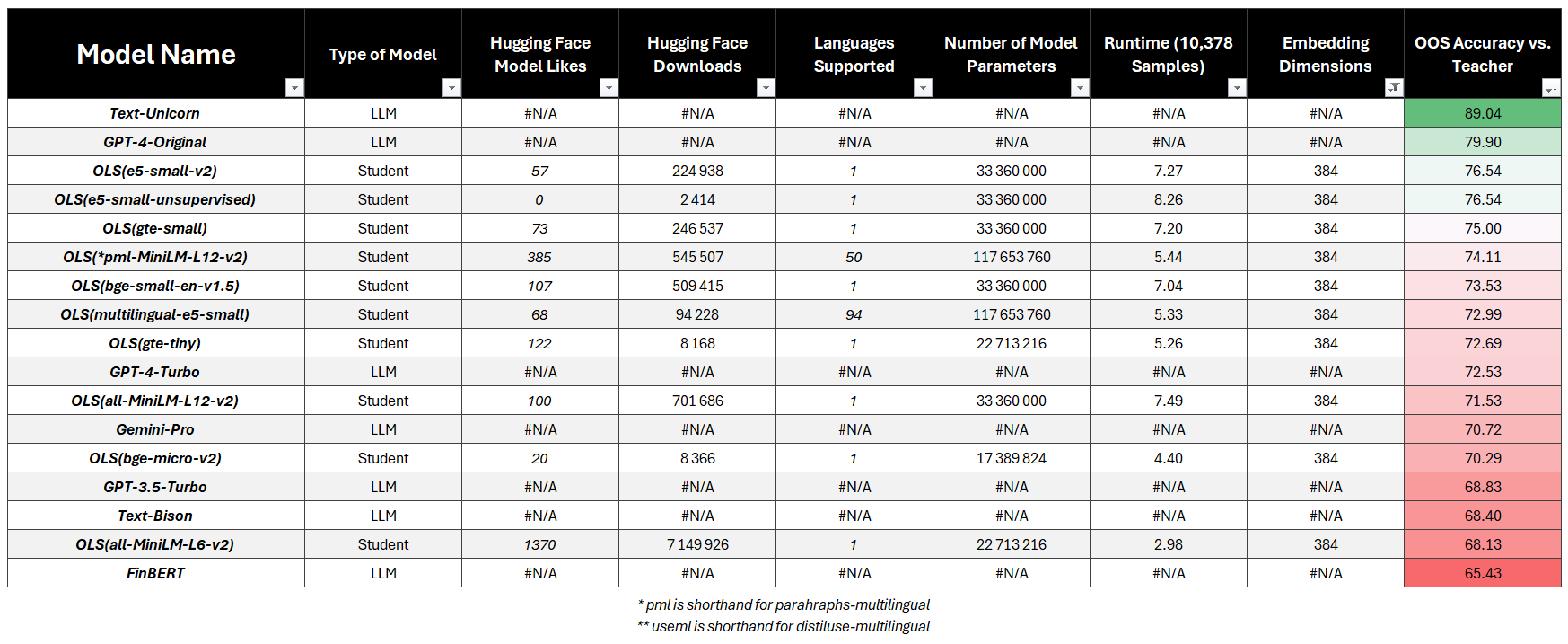
• LLM Targets:
  • PaLM-2 Unicorn (89.04%)
  • GPT 4 Original (79.90%)
• Students:
  • Best: e5-small-v2 (76.54%)
  • Fastest: all-MiniLM-L6-V2 (68.13%)
  • Most Popular: all-MiniLM-L6-V2 (68.13%)

768-Dimensional Vectors

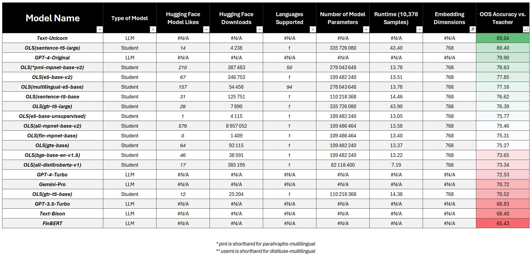
• LLM Targets:
  • PaLM-2 Unicorn (89.04%)
  • GPT 4 Original (79.90%)
• Students:
  • Best: sentence-t5-large (80.40%) 🏆
  • Fastest: all-distilroberta-V1 (73.34%)
  • Most Popular: all-mpnet-base-v2 (75.46%)

1024-Dimensional Vectors

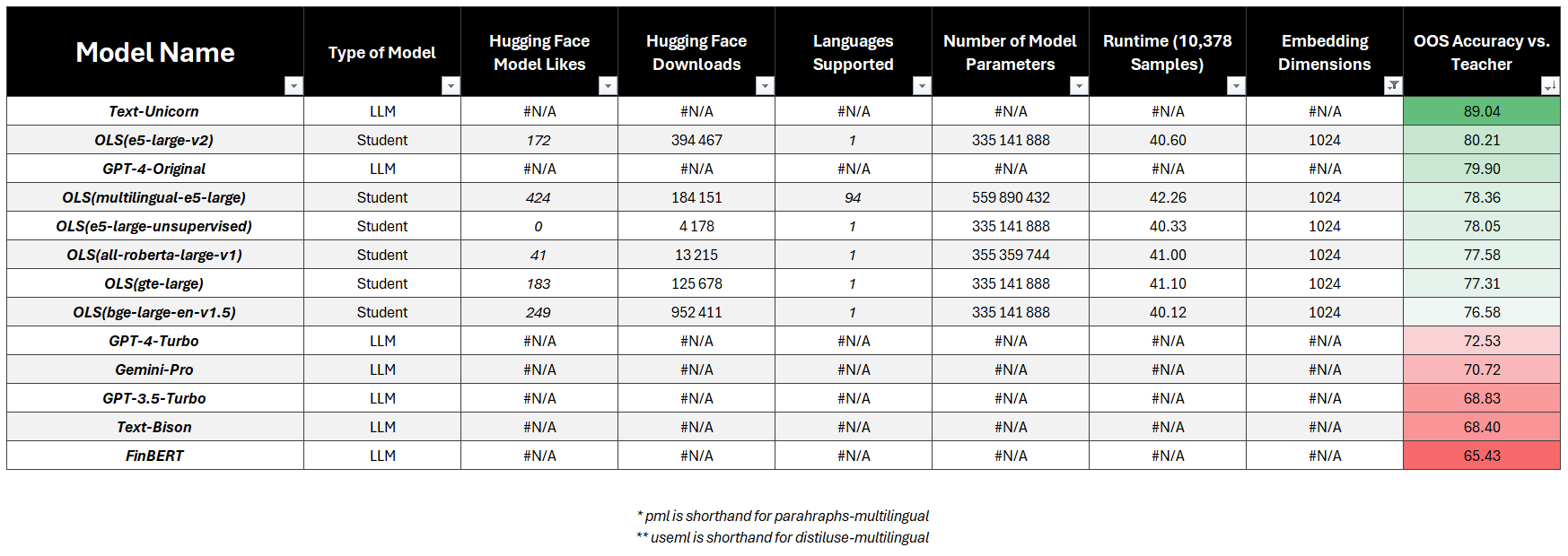
• LLM Targets:
  • PaLM-2 Unicorn (89.04%)
  • GPT 4 Original (79.90%)
• Students:
  • Best: e5-large-v2 (80.21%) 🏆
  • Fastest: bge-large-en-v1.5 (76.58%)
  • Most Popular: bge-large-en-v1.5 (76.58%)

Multilingual Vectors

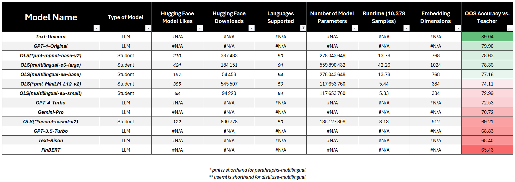
• LLM Targets:
  • PaLM-2 Unicorn (89.04%)
  • GPT 4 Original (79.90%)
• Students:
  • Best: paraphrase-multilingual-base-v2 (78.63%)
  • Fastest: multilingual-e5-small (72.99%)
  • Most Popular: distil-use-multilingual-cased-v2 (69.21%)

Conclusions

You might be sitting there thinking, "Damn Stuart, that sounds like a hell of a lot of work, is it worth it?". That's a fair question. If you're dealing with small data, this is overkill. However, if you are like us, and you're dealing with big data, then my answer is a resounding "Yes!". And there are four reasons for that:

It's Better

First and foremost, we found two student models that outperform GPT-4 when compared against the teacher ensemble. These two models were🥇 sentence-t5-large (80.40%) and 🥈 e5-large-v2 (80.21%). Remember the ensemble model achieved 90% agreement with human labels so this is meaningful.

It's Cheaper

Second, in our previous post we showed that classifying the sentiment of 10 million news stories would cost an eye-popping \$92,000 using GPT-4. With this student model, which beats GPT-4, we can do the same for \$0.00 marginal cost. In fact, using that $92,000 we could probably buy three Nvidia H100's.

It's Faster

Third, using GPT-4 it takes about ~0.5 seconds to classify the sentiment of one news story. 10 million news stories would take 57 compute days. Using the best students models it takes ~0.005 seconds to classify the sentiment of one news story. 10 million stories would take less than 1 compute day to complete.

It's Reusable

Finally, you shouldn't see this as a once-off exercise. This is the data science equivalent of a design pattern. It can be used and reused over and over again to solve problem after problem. Between ourselves and Alphix Solutions we are using this data design pattern to solve a variety of problems like -

1. Sentiment Classification (Positive, Neutral, Negative)
2. Tense Classification (Past, Present, Future)
3. News Classification (M&A, Legal, Results, etc.)
4. Brand Safety Classification (Safe, Unsafe)
5. Beat Classification (Opinion, Formal, Investigative)
6. Political Bias Classification (Left, Centrist, Right)
7. Statement Classification (Forward or Backward looking)
8. IAB Website Classification (Over 700 categories!)

And that's a wrap. If you enjoyed this post and would like to see more content like this, please subscribe to our blog. The appendix below contains the code and dataset you need in order to replicate these results for yourself 🤓.

Appendix

This whole analysis was performed in just 198 lines of Python code (less if you don't count lists of model names). Here's everything you need:

import datetime as dt
import json

import numpy as np
import pandas as pd
from sentence_transformers import SentenceTransformer
from sklearn.linear_model import LinearRegression
from sklearn.model_selection import train_test_split

# Store experiment results.
experiment_results_dict = {}

# Specify the dataset we want to work with.
dataset = "small/nosible-news-small"

with open(f"{dataset}.json") as f:
    # Load the raw data (headlines, etc.)
    news_data: dict = dict(json.load(f))

with open(f"{dataset}-labels.json", "r") as f:
    # Load the labels assigned by various LLMs.
    news_labels: dict = dict(json.load(f))

# Loop through each news story in the dataset.
for key, labels in news_labels.items():
    ensemble_score = sum(
        [
            # Get the ensemble's score.
            labels["Text-Unicorn"],
            labels["GPT-3.5-Turbo"],
            labels["GPT-4-Original"],
            labels["Sigma"],
            labels["Text-Bison"],
        ]
    )

    news_data[key].update(
        {
            # Add the teacher to the dataset.
            "Teacher": ensemble_score,
            **labels  # Add raw LLMs too.
        }
    )

sentences = []

for key, document in news_data.items():
    # Create a sentence for each of the news stories we want to train on.
    sentences.append(f"{document['Headline']}. {document['Description']}")

for model_ix, model_name in enumerate(
        [
            # Hugging Face sentence-transformer models. This list goes from models with the
            # fewest parameters (fastest) to the model with the most parameters (slowest).
            "TaylorAI/bge-micro-v2",
            "TaylorAI/bge-micro",
            "sentence-transformers/all-MiniLM-L6-v2",
            "sentence-transformers/all-MiniLM-L6-v1",
            "TaylorAI/gte-tiny",
            "sentence-transformers/all-MiniLM-L12-v2",
            "sentence-transformers/all-MiniLM-L12-v1",
            "BAAI/bge-small-en-v1.5",
            "thenlper/gte-small",
            "intfloat/e5-small-v2",
            "intfloat/e5-small-unsupervised",
            "sentence-transformers/all-distilroberta-v1",
            "BAAI/bge-base-en-v1.5",
            "thenlper/gte-base",
            "intfloat/e5-base-v2",
            "intfloat/e5-base-unsupervised",
            "mukaj/fin-mpnet-base",
            "sentence-transformers/all-mpnet-base-v2",
            "sentence-transformers/all-mpnet-base-v1",
            "sentence-transformers/sentence-t5-base",
            "sentence-transformers/gtr-t5-base",
            "intfloat/multilingual-e5-small",
            "sentence-transformers/paraphrase-multilingual-MiniLM-L12-v2",
            "sentence-transformers/distiluse-base-multilingual-cased-v1",
            "sentence-transformers/distiluse-base-multilingual-cased-v2",
            "intfloat/multilingual-e5-base",
            "sentence-transformers/paraphrase-multilingual-mpnet-base-v2",
            "BAAI/bge-large-en-v1.5",
            "thenlper/gte-large",
            "intfloat/e5-large-v2",
            "intfloat/e5-large-unsupervised",
            "sentence-transformers/sentence-t5-large",
            "sentence-transformers/gtr-t5-large",
            "sentence-transformers/all-roberta-large-v1",
            "intfloat/multilingual-e5-large",
        ]
):
    # Load the sentence transformer model.
    encoder = SentenceTransformer(
        model_name_or_path=model_name,
        trust_remote_code=True
    )

    # Count the number of parameters that are in the model.
    parameters = sum(p.numel() for p in encoder.parameters())

    # Start the timer for this model.
    t0 = dt.datetime.utcnow()

    # Generate the embeddings.
    embeddings = encoder.encode(
        sentences=sentences,
        show_progress_bar=False
    )

    # Get the dimensionality of the model.
    dimensionality = embeddings.shape[1]

    # Get the runtime that it took to encode all sentences.
    runtime = (dt.datetime.utcnow() - t0).total_seconds()

    # Create input and output DataFrames for distillation.
    out_df = pd.DataFrame.from_dict(data=news_data, orient="index")
    in_df = pd.DataFrame(data=embeddings, index=out_df.index)

    # Split the data into a training and a validation set.
    x_train, x_test, y_train, y_test = train_test_split(
        in_df, out_df, test_size=0.25, random_state=42
    )

    # Get the out-of-sample teacher labels (Ensemble).
    teacher_llm = y_test["Teacher"].values
    teacher_llm_classes = np.zeros(len(teacher_llm))
    teacher_llm_classes[teacher_llm <= -1] = -1
    teacher_llm_classes[teacher_llm >= 1] = 1

    # If this is model #1.
    if model_ix == 0:

        for prev_model_name in [
            'TextBlob-0.10',
            'TextBlob-0.20',
            'TextBlob-0.30',
            'VADER-0.10',
            'VADER-0.20',
            'VADER-0.30',
            'Flair-0.50',
            'Flair-0.75',
            'Flair-0.95',
            'Sigma',
            'FinBERT',
            'FinBERT-Tone',
            'Text-Bison',
            'Text-Unicorn',
            'Gemini-Pro',
            'GPT-3.5-Turbo',
            'GPT-4-Turbo',
            'GPT-4-Original',
        ]:
            # Get the predictions of the previous model on the test set.
            y_test_llm_classes = y_test[prev_model_name].values
            y_test_llm_sames = (y_test_llm_classes == teacher_llm_classes)
            y_test_llm_matches = np.sum(y_test_llm_sames)
            test_accuracy = y_test_llm_matches / len(y_test_llm_sames) * 100
            print(f"{prev_model_name} : {test_accuracy:.2f}%")

            # Add the previous models to the results.
            experiment_results_dict[prev_model_name] = {
                "Parameters": np.nan,
                "Runtime": np.nan,
                "Dimensions": np.nan,
                "Accuracy": test_accuracy,
            }

    # Fit the linear regression on the embeddings.
    linear_regression = LinearRegression()
    linear_regression.fit(x_train.values, y_train["Teacher"].values)

    # Use the linear regression to predict the teacher sentiment scores.
    y_pred_test = linear_regression.predict(x_test.values)

    # Turn the sentiment scores into labels {-1, 0, +1}.
    y_pred_test = y_pred_test.flatten()
    y_pred_test_classes = np.zeros(len(y_pred_test))
    y_pred_test_classes[y_pred_test <= -1] = -1
    y_pred_test_classes[y_pred_test >= 1] = 1

    # Calculate the out-of-sample accuracy of the student model.
    y_test_sames = (y_pred_test_classes == teacher_llm_classes)
    y_pred_matches = np.sum(y_test_sames)
    test_accuracy = y_pred_matches / len(y_test_sames) * 100
    print(f"OLS({model_name.split('/')[-1]}) : {test_accuracy:.2f}%")

    # Add the student model to the results with the OLS naming convention.
    experiment_results_dict[f"OLS({model_name.split('/')[-1]})"] = {
        "Parameters": parameters,
        "Runtime": runtime,
        "Dimensions": dimensionality,
        "Accuracy": test_accuracy,
    }

# Convert the results into a pandas DataFrame and save it to a CSV file.
results_df = pd.DataFrame.from_dict(experiment_results_dict, orient="index")
results_df.to_csv("Results.csv")

This code relies on two datafiles which should sit in the same directory as this Python script. These files contain a small dataset of news stories and labels.

About Nosible

If you're an asset manager looking for ways to add artificial intelligence and large language models into your investment process, we would absolutely love to hear from you. This post, whilst impressive, is just a small demonstration of our full capabilities. The real magic happens at scale and in the intersection. For example, using our index we can extract the rolling 3-month sentiment across all forward-looking statements made about each and every US listed company going back 10 years. If that sounds cool, drop me a line. My email is stuart@nosible.com 👋